
In a recent collaboration with experts from natural and medical sciences, we show how Invertible Neural Networks can help us deal with the ill-posed inverse problems that often arise in these fields. This page aims to provide an intuitive introduction to the idea.
Click on the thumbnails to jump to different sections.
A quick introduction to Invertible Neural Networks
Ambiguous Inverse Problems and how we can solve them
Verifying our approach with a simple toy example
Application to data from two real-world problems

Some closing thoughts and a look at what’s next
1. Invertible Neural Networks
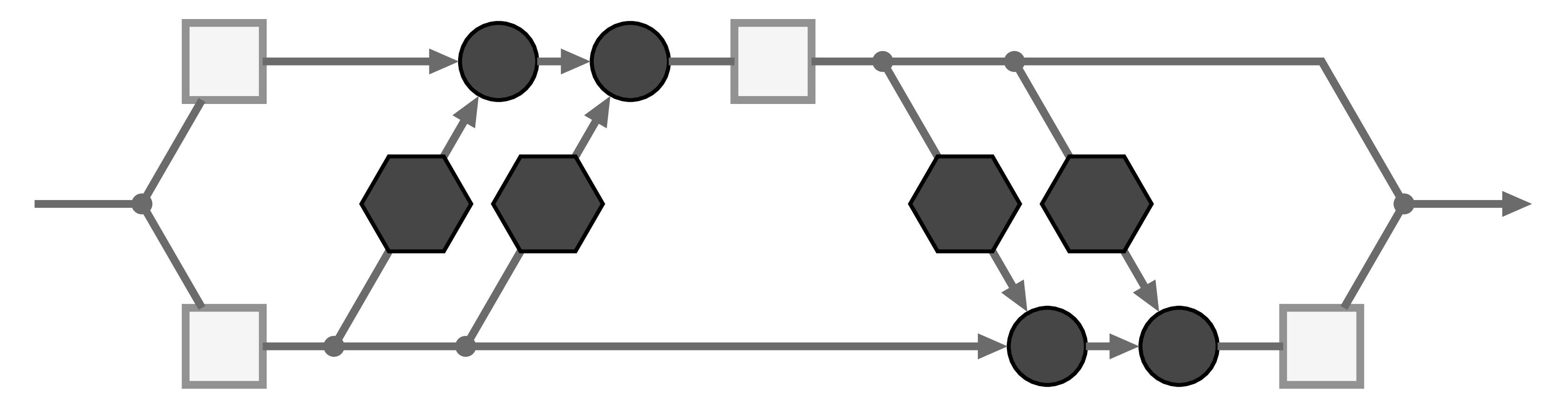
The basic building block of our Invertible Neural Network is the affine coupling layer popularized by the Real NVP model. It works by splitting the input data into two parts ![[\mathbf{u}_1, \mathbf{u}_2]](https://quicklatex.com/cache3/a0/ql_695ade0b4182309aae2a8e5f2a9730a0_l3.png "Rendered by QuickLaTeX.com") , which are transformed by learned functions
, which are transformed by learned functions  and coupled in an alternating fashion like so:
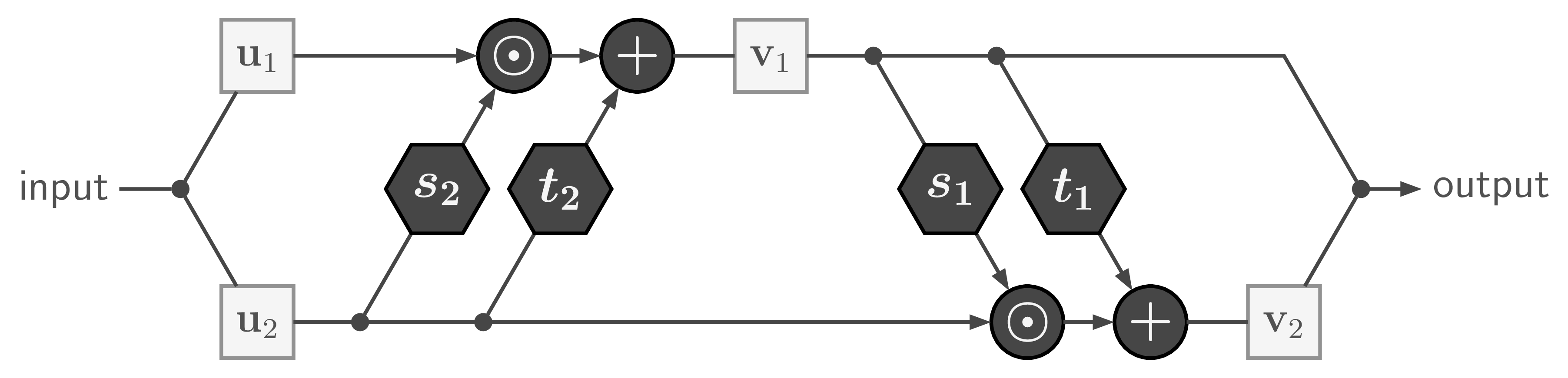
where  is element-wise multiplication. The output is just the concatenation of the resulting parts
 ![[\mathbf{v}_1, \mathbf{v}_2]](https://quicklatex.com/cache3/62/ql_8a6611a2e198b83b11e0e6555ccffb62_l3.png "Rendered by QuickLaTeX.com") .
.
With only minor rearrangements, we can recover from to compute the inverse of the whole affine coupling layer:
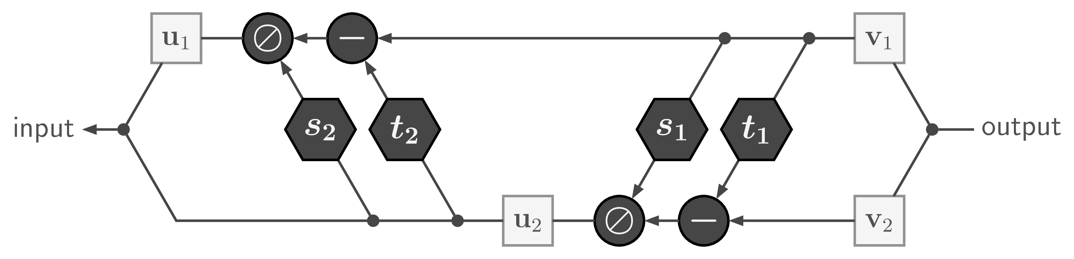
with  being element-wise division.
Like in many scenarios, direct division can lead to numerical problems. So in practice we use the exponential function and clip extreme values of  , which leads to a forward pass of the form

with the inverse given by

To construct deep invertible networks, we can simply chain these affine coupling layers much like ResNet blocks.
Crucially, the transformations  and
and  themselves need not be invertible and can be represented by arbitrary neural networks, which are trained by standard backpropagation along the computation graph. What’s more, invertibility allows us to apply loss functions for the forward pass and the inverse pass at the same time, and compute gradients for and from either direction – an opportunity we will exploit later on.
Rules how to assign data to the upper or lower lane (i.e. how to split the input into  and
and  ) are still an active area of research. In a fully connected network, one typically splits in a random (but fixed!) way, and changes the assignment from layer to layer. When the data have spatial structure (think of images) and the transformations use a convolutional architecture, one usually divides along the channel dimension in every pixel. Recently, Kingma and Dhariwal proposed to learn the assignment.
So where’s the catch?
The big constraint for this kind of scheme is that input and output of each module must have the exact same dimensionality. INNs look like auto-encoders whose codes have the same size as the original data. While this appears strange at first, the encoding  can still disentangle complex data distributions
  to the point where surprising data manipulations become possible. Look at the demo of the Glow network to get an idea of the method’s potential when applied to images.
2. Ambiguous Inverse Problems
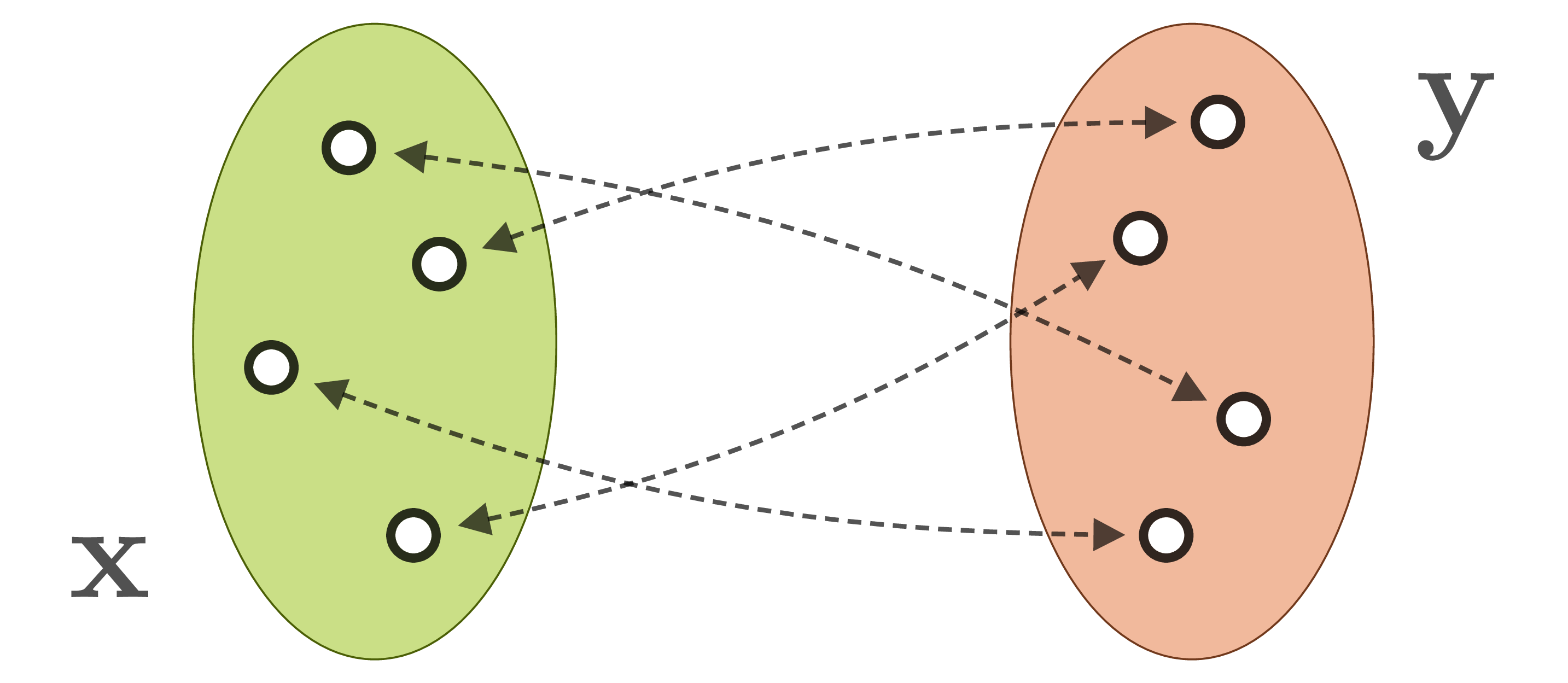
When we observe a system in the natural world, we generally can’t measure its internal parameters  directly. Instead, our observations are produced by a forward process, which translates system parameters into observable quantities. Often, the forward process is well understood, but incurs a loss of information. For example, when the 3D world is projected onto a camera image, information about depth, surface normals, light source positions etc. is lost. As a result, different system states are mapped onto identical observations :
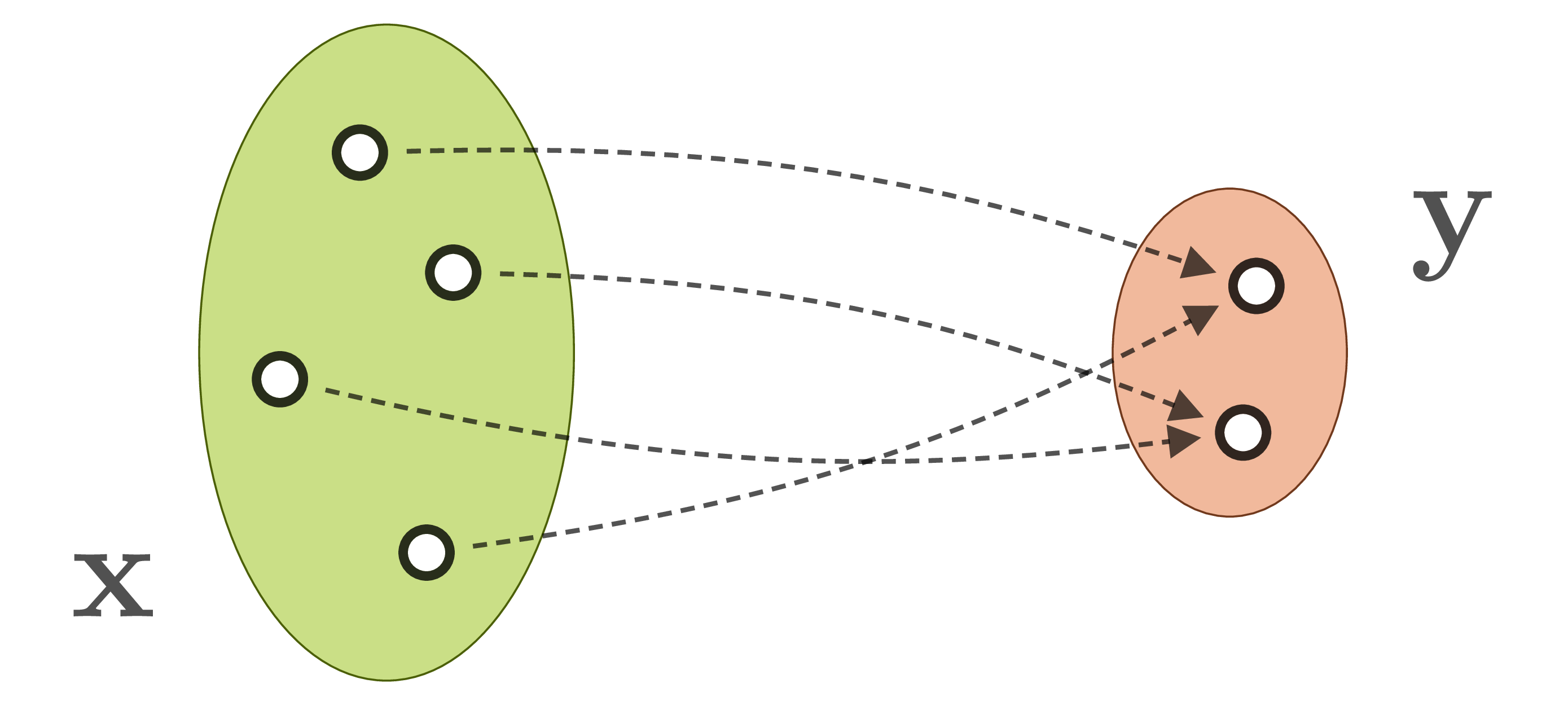
The inverse process, which we need to infer parameters from observations , is therefore ambiguous and ill-posed, and its explicit modeling intractable. Instead, one applies statistical inference techniques to express the ambiguities in form of conditional probabilities  ). Classical Bayesian methods for this problem like MCMC sampling or Approximate Bayesian Computation employ different sampling approaches, but quickly become very expensive even for moderate real-world problems.
Can we learn it?
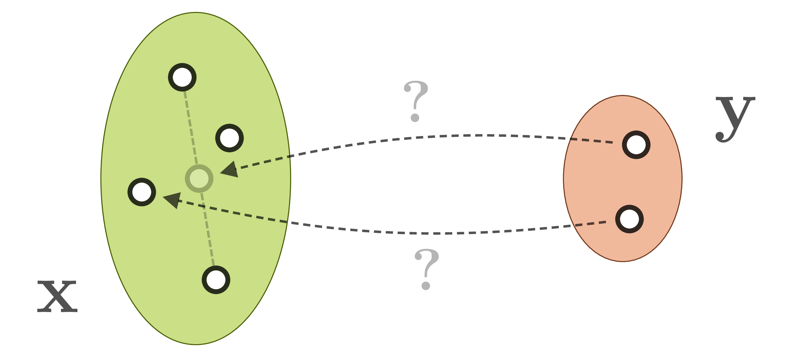
In many domains, experts already posses sophisticated models for the forward process, and they can easily generate large data sets of matching state/observation pairs  by simulation. An abundance of data makes machine learning, and especially neural networks, a promising approach. But direct supervised learning of
  is problematic for ambiguous inverse problems. Using standard network architectures, the learned mapping will either pick only one of the eligible for a given , or even worse, will form an average between multiple correct, but incompatible inverses:
We actually want our network to learn the full posterior distribution  . We could learn to predict fitting parameters of a simple distribution, or make the network weights themselves variational, or even both, but in any case this will restrict us to one chosen (simple) family of distributions. We could also turn to conditional GANs, but these are notoriously difficult to train and often suffer from hard-to-detect mode collapse.
Resolving the ambiguity
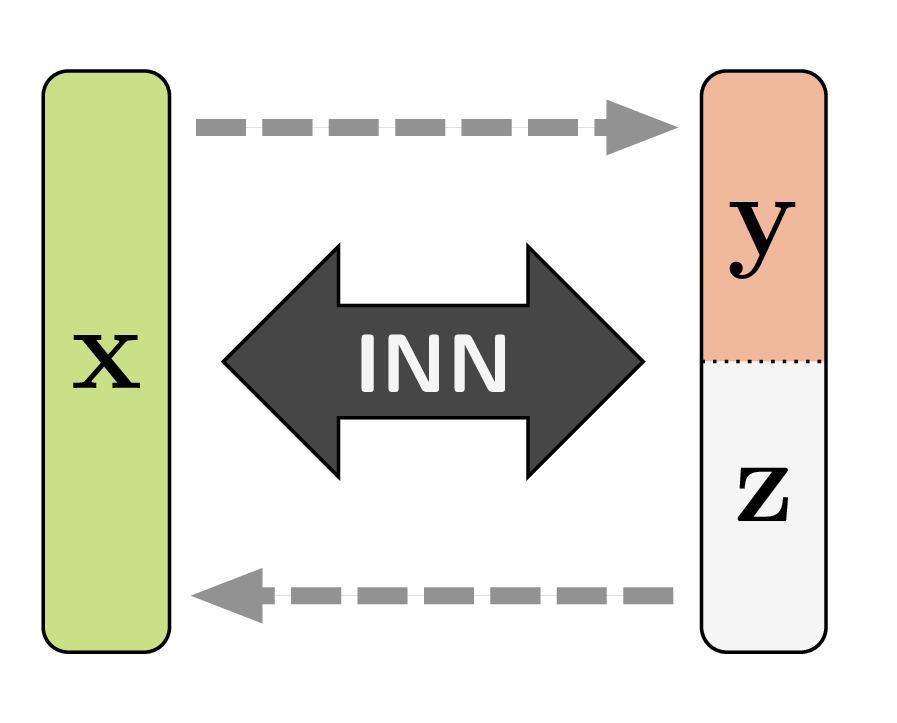
What we propose to do instead is to introduce additional latent variables  which capture the information that would otherwise get lost in the forward process. Consequently,
 ![\mathbf{x} \leftrightarrow [\mathbf{y}, \mathbf{z}]](https://quicklatex.com/cache3/76/ql_c662d20d4bf63bc77c7994208669fd76_l3.png "Rendered by QuickLaTeX.com") becomes a bijective mapping:
becomes a bijective mapping:
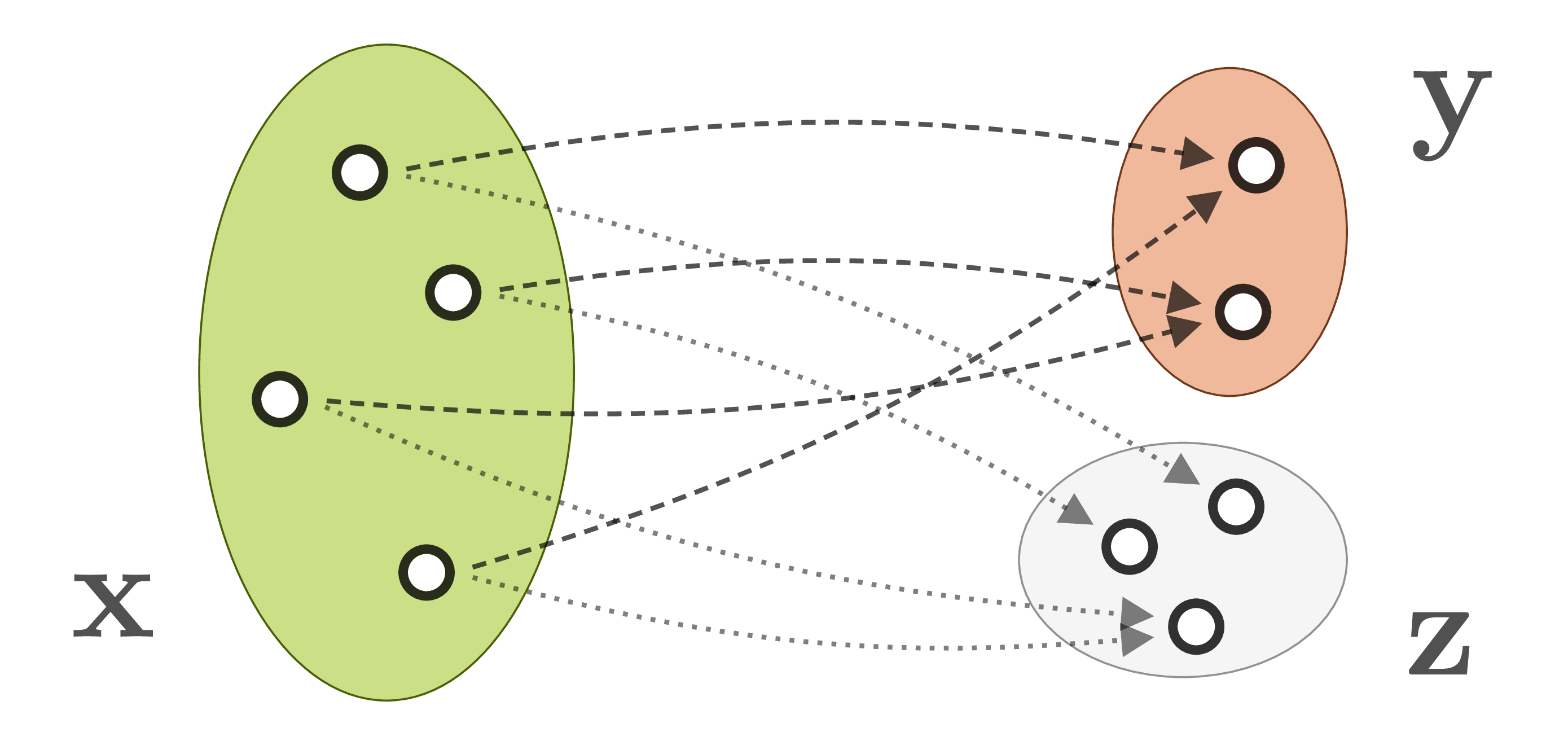
And this bijective mapping is a great fit for the Invertible Neural Networks we discussed in the beginning! Of course we have to make sure that and ![[\mathbf{y}, \mathbf{z}]](https://quicklatex.com/cache3/b5/ql_e49838c0baa504ab886e6ad25cd40fb5_l3.png "Rendered by QuickLaTeX.com") have the same total dimensionality. But it turns out that we can cheat this rule, in a way, by artificially increasing the dimensionality of either side with zero padding. We can even pad both sides, which means that intermediate representations have higher dimensionality as well, making the model more powerful.
have the same total dimensionality. But it turns out that we can cheat this rule, in a way, by artificially increasing the dimensionality of either side with zero padding. We can even pad both sides, which means that intermediate representations have higher dimensionality as well, making the model more powerful.
Assume for a moment that we have an invertible network which perfectly reproduces the simulation of the forward process, and arranges to follow some simple distribution (e.g. standard normal). With this, we can approximate the distribution just by repeatedly sampling and running the inverse pass of the network, i.e. ![[\mathbf{y}, \mathbf{z}] \rightarrow \mathbf{x}](https://quicklatex.com/cache3/5f/ql_e5f049edbb9a32228809d3401e58505f_l3.png "Rendered by QuickLaTeX.com") . In other words, has been reparametrized into a deterministic function
. In other words, has been reparametrized into a deterministic function  with noise variable . If you think this sounds like a conditional GAN, you are absolutely right. At test time, it’s the same thing! But the invertible architecture allows for a completely different training scheme, with some distinct advantages.
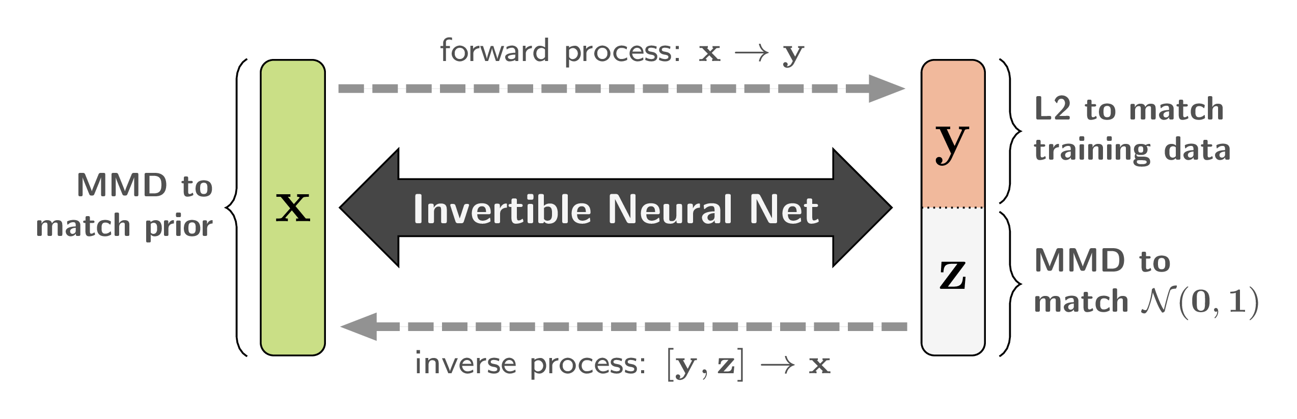
Because of the bijective nature of our network, we can train it to solve the well-posed forward process  in a supervised manner, instead of the ill-posed inverse process. We require the latent variables to be independent of , and to follow an easy-to-sample-from distribution, like
  . Both conditions can be achieved with a Maximum Mean Discrepancy (MMD) loss, which matches two distributions by comparing samples.
As a mild form of regularization, we also apply MMD between from our model (marginalized over all and ) and the prior represented by the training data. Here, we make use of the previously mentioned bi-directional training to accumulate gradients from loss terms on either end of the network. In the same way we could add a GAN-like discriminator loss on . But in our applications so far, MMD turned out to be sufficient, so we can avoid the troubles of adversarial training. Finally, if we use zero padding for the input or output, we put a simple sparsity-enforcing loss on the dimensions in question.
Intuitively, our network learns to mimic the simulation, while splitting information about the ambiguity of its inverse off and transforming it into normally distributed latent variables. When we learn this forward transformation, we get the inverse for free, thanks to the invertible construction of our network. It is not even necessary to make any assumptions about or the target distribution . Also, since each training pair  must be mapped to some position
  in latent space, it can be recovered when sampling for the inverse direction. We observe this to be a strong mechanism against mode collapse.
3. Does it work? A Toy Example
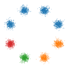
To check how well we can recover the shape of , consider the following set of toy problems. Our parameters are the 2D coordinates of points distributed according to a Gaussian Mixture Model with eight components, arranged in a circle. Samples from this -distribution are colored depending on which mode they were drawn from – we take these color labels to be our measurements . We test three different measurement “labellings”: each mode has a different color (left), some colors are shared (middle) or all modes have the same color (right). These correspond to progressively more ambiguous forward processes.
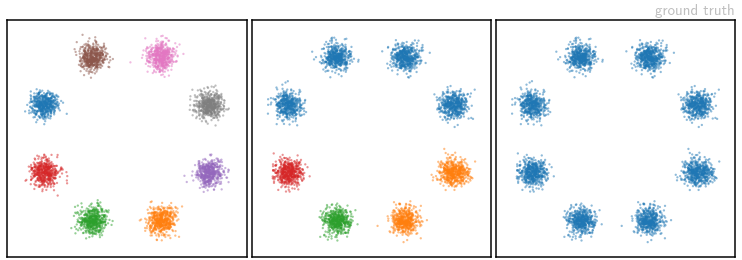
The image above shows samples from the ground truth setup of the three different labellings. Corresponding samples from our network’s learned posterior distributions are shown in the video below, as they evolve over the course of training:
(click on video to play/pause/restart – or view final result directly)
All three experiments were performed with the same model architecture, all losses weighted equally. It is easy to see that our Invertible Neural Network is able to reproduce the original distributions reliably and accurately. In the paper’s supplemental material we also show results obtained by various established methods. Most of them struggle with this toy example when afforded the same number of trainable parameters.
Structure of the latent space
For the experiments shown above, we only used a two-dimensional latent space. This way we can visualize as an image how the model is using , given a specific label . For each coordinate  in latent space, we run
 ![[\mathbf{y}, \mathbf{z}_{i}]](https://quicklatex.com/cache3/85/ql_9e51b90d6749a26f1b640d3a2d293985_l3.png "Rendered by QuickLaTeX.com") through the inverse pass of our model to obtain a sample
through the inverse pass of our model to obtain a sample  , then color the corresponding pixel as follows: The hue depends on the mode in -space that is closest to. The intensity depends on how far away is from that mode.
For the label ![\mathbf{y} = \text{\bfseries\color[rgb]{1.0,0.5,0.05}orange}](https://quicklatex.com/cache3/12/ql_cf18c112fb03a46d21eeeaf6c9c95812_l3.png "Rendered by QuickLaTeX.com") in the middle setting, the latent space of our converged model looks like this:
in the middle setting, the latent space of our converged model looks like this:
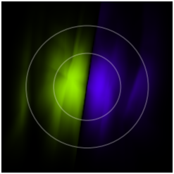
The colors used here have nothing to do with the the ones used as -labels before. The two circles mark the areas that contain 50% and 90% of the probability mass of the Gaussian latent prior  , respectively. We can see that -space is divided into two equally sized regions, corresponding to the two orange modes in the middle setting.
We can also compare the layout for ![\mathbf{y} = \text{\bfseries\color[rgb]{0.12,0.47,0.71}blue}](https://quicklatex.com/cache3/df/ql_e0cdc1c646ac3b70fd29b6f2fa4cb2df_l3.png "Rendered by QuickLaTeX.com") in all three settings. The video below shows how the latent space visualization develops over the entire course of training:
in all three settings. The video below shows how the latent space visualization develops over the entire course of training:
(click on video to play/pause/restart – or view final result directly)
4. Where can we apply this?
Ambiguous inverse problems as described above pop up in many places, and often enough scientists can simulate a system better than they can effectively observe it. We looked at two such problems, the first coming from medical science.
In medical science
To make optimal decisions during minimally invasive surgery, doctors ideally want to know a number of local properties of the tissue they operate on, such as oxygen saturation, layer thickness and blood flow. However for practical reasons, they can only inspect the tissue’s surface with a tiny multispectral camera. Many different configurations of the tissue parameters can result in the same spectral response , and so they end up with an ambiguous inverse problem. Using data from high-quality simulations of this process, we applied our new method to tackle this problem.
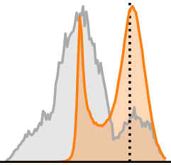
The following animation shows how we reconstruct the posterior with our fully trained Invertible Neural Network by sampling more and more instances of for a single given observation .
(click on video to play/pause/restart – or view final result directly)
Each panel develops the marginal posterior  for a single parameter
  , shown in orange. The gray areas show the prior over the whole date set for context. The dotted lines are ground truth values from an actual associated with in the test set.
We can see that the network is very certain (and apparently spot-on) about oxygen saturation. For blood density, the posterior is visibly lopsided in order to avoid values outside of the prior’s support. Most interestingly, in the last two panels, posterior and prior are practically identical. This is our network telling us that we simply cannot derive any information about these parameters from our spectral measurements .
Details about the data set and experiment can be found in the paper. There we also show that we can find correlations between the parameters’ posteriors, which are especially interesting to domain experts.
In astrophysics
A very similar problem arises in a branch of astrophysics that explores the life cycle of star clusters in interstellar gas clouds. The internal parameters of such systems, and simulations thereof, are very complex and interact a lot over time. But observation of real objects is again essentially limited to snapshots of the emitted light spectrum, introducing strong ambiguity. As before, we trained our network on data from state-of-the-art simulations.
And again, we can sample from the latent space to generate marginal posterior distributions with our fully trained model, given an observation :
(click on video to play/pause/restart – or view final result directly)
Colors have the same meaning as before. The peculiar shape of the prior here is due to the very dynamic behavior of star cluster simulations over time.
In this scenario, we actually find distinctly multi-modal distributions for some parameters . These multiple modes, combined with the correlation between marginal posteriors, offer great insights into the system. We can for example say that this specific observation either corresponds to a young cluster with large expansion velocity, or to an older system that expands slowly.
5. Closing thoughts
An open question, which we share with e.g. Autoencoder architectures, is how to determine the intrinsic dimension of a task or dataset. For best results, should be neither smaller nor larger than this.
The special structure of the coupling layers in Invertible Neural Networks may preclude direct application of some other architectural tricks. On the flipside, it offers a unique memory/computation trade-off as we don’t need to store activations from the forward pass for backpropagation. We are however not making use of this in our current work.
Overall, the permutation of variables between subsequent (blocks of) coupling layers seems to be a crucial point. Without permutation, variables  from the two streams
  can only interact via coupling, and never within the same subnetwork. A generalization of the simple shuffle we use is the main technical contribution of the brand new Glow framework.
Several previous works have proposed training networks for both directions of a task, some even with coupled weights. But we are not aware of any setting where loss functions were placed on either end of one and the same network [Update: Flow-GAN does so with an invertible generator network]. This truly bi-directional training could open up many possibilities, and we are excited to see where else it might be used.
Further Reading
- Dinh, Laurent, Jascha Sohl-Dickstein, and Samy Bengio. “Density estimation using Real NVP.” arXiv preprint arXiv:1605.08803 (2016).
- Kingma, Diederik P., and Prafulla Dhariwal. “Glow: Generative Flow with Invertible 1×1 Convolutions.” arXiv preprint arXiv:1807.03039 (2018).
- Schirrmeister, Robin Tibor, et al. “Training Generative Reversible Networks.” arXiv preprint arXiv:1806.01610 (2018).
- Jacobsen, Jörn-Henrik, Arnold Smeulders, and Edouard Oyallon. “i-RevNet: Deep Invertible Networks.” arXiv preprint arXiv:1802.07088 (2018).